
I have my MATLAB laser simulation pretty fleshed out. It supports continuous wave and Q-switched laser designs with and without intracavity second harmonic generation. It takes into account a whole pile of different parameters. Examples:
Fiber collimator optics, spot size calculations, Raleigh length and transmission losses.
Mirror losses, optimal output coupler reflectance, and effective output coupling when using SHG.
Thermal lensing characteristics and how lensing affects beam size, saturable absorber behavior, SHG conversion and maximum power output before the beam is destabilized.
Average and peak output power, pulse repetition rate and pulse width.
SHG conversion chacteristics.
I also have several laser models defined. The three main models are the laser I built, a test laser on my workbench and the “new” laser design. These will be referred to as the 2020 laser, the bench laser and the 2023 laser.
2020 Laser Observations
The goal is to change the 2020 laser design to be Q-switched. Starting with that design with no second harmonic generation, I added a saturable absorber as a Q-switch. I read a great paper on Q-switching that recommended the beam waist inside the Q-switch be 20-30x smaller area than the waist in the gain medium. Starting with that, I modeled several initial transmissivities of Cr:YAG:

I am trying to maximize average power output here, so I will choose the .9 absorber. I can play with this later in the model and see how it affects average and peak output power.
To calculate the power for Q-switching, I converted my simulation over to being based completely on the population inversion of the laser crystal. I have an algorithm that can calculate the initial and final inversion for both continuous wave and pulsed operation. MATLAB was helpful here but I’m not sure I’m using it correctly. To calculate initial and final inversions there are a few equations that have to be simultaneously solved. The tricky part is one of the equations is transcendental:
$$ n_i - n_f = n_t ln \left( \frac{n_i}{n_f} \right) $$
This equation constrains the relationship between initial and final inversions but it has no algebraic solution. I am having MATLAB solve this by providing a guess based on an infinite pulse duration, and if I don’t get a solution I continue to divide the guess by 10. There’s probably a better (and faster) way.
I the took this Q-swiched laser at max power and added a KTP crystal for second harmonic generation. I modeled a range of beam waists inside the crystal and I modeled a 5mm long crystal and a 10mm long crystal. The resulting power output is interesting:

Wait..what? Second harmonic conversion inside KTP is pretty complex. As the wave propagates in the crystal sometimes it is re-absorbed and interacts with the lattice to produce some chaotic results. The second harmonic conversion efficiency is calculated as follows:
$$\eta = \eta_m sn^2 \left[ \sqrt{\frac{\eta_0}{\eta_m}}, \eta_m^2 \right]$$
Where:
$$ \eta_0 = C^2L^2I_\omega, $$
$$ \eta_m = 1 + \left( \frac{\delta^2}{2\eta_0} \right) - \sqrt{\left[ 1 + \left( \frac{\delta^2}{2\eta_0} \right) \right] ^2 - 1}, $$
$$ C = 5.46 \frac{d_{eff}}{\lambda_0n_0^{3/2}}, $$
$$ \delta = \frac{\Delta kL}{2}, $$
$$ \Delta k = \left( \frac{\beta_{\theta}}{n_0}\right) \left( \frac{\theta}{2} \right) $$
Some of this math, like ‘sn(u, m)’ (which is the Jacobi elliptic function) is stuff I’ve never seen. Luckily MATLAB has. Calculating actual conversion efficiency when the crystal is inside the laser cavity is further complicated because the crystal conversion is related to the intensity, but as the crystal gets more efficient due to higher intensity, this leaks more green light out of the cavity and lowers the intensity inside the cavity. This lowers the conversion rate so you end up with a feedback loop that eventually reaches steady-state.
MATLAB has some cool tricks up its sleeve for this. You can write functions that are just program code, and combine them together like any normal program. But then you can run a solver over the algorithm to find the inputs. Here’s an example:
function value = Foo(a, b)
    value = a + b;
end

function value = Bar(a)
    value = Foo(a, a + 5) * 2;
end

function Test()
    fprintf('%f', Bar(5)); % prints 30

    syms a;
    eqn = 30 == Bar(a);
    fprintf('%f', vpasolve(eqn)); % prints 5
end
That’s really handy and I was able to scale that up to solving for the steady state for the SHG conversion. Neat.
The summary here is that you don’t want the intensity into the KTP to be high enough that you start to dip into that chaotic region. The sweet spot is that last high peak. Also, the 5mm and 10mm crystals produce effectively the same output, but optimize for different intensities.
Cavity Design
The above observations can be applied to the design of the laser cavity:
You want as large a waist as possible in the gain crystal to limit thermal lensing.
You want the waist in the Cr:YAG crystal to have an area about 20-30x smaller than the gain.
You want the waist in the KTP crystal to have an area about 5x smaller than the gain.
The design I came up with looks like this:

I iterated on this for a while, bouncing between Rezonator to get the design parameters to MATLAB to calculate the results and then to Fusion 360 to model the design and make sure it was buildable. When I first started this design it looked fantastic. It dealt very well with thermal lensing, and by sliding the Cr:YAG along the focal point between two curved mirrors I could dial in the pulse repetition rate.
Unfortunately I didn’t account for mirror angles. In order to build a cavity that looks like this in a small space you have to fold it up and you need six mirrors. Two of them are curved and are at angles. A beam on a curved mirror that is at an angle becomes an ellipse. I used a little simple trigonometry (Resonator — thank you for LUA scripting) to factor this in. The mirrors I’m using are 1” in diameter, and once you factor in the mounts the closest I can get each “row” of the resonator is about 2”. That’s not great for those ellipses. I minimized where I could and went with smaller 1/2” mirrors where I could, to arrive at this basic resonator design. It’s got pretty tight tolerances:

The parts to implement this are costly. It adds up to over $3000.00 in new parts, and that’s not including seven components that need to be custom made. Aligning it will be a chore too. Some of the distances between mirrors need to be accurate to the millimeter, and any change to their distance lengths requires re-aligning the whole thing so any iteration is very time consuming.
I have ordered the bare minimum of new parts to test if this design works.
Revisiting Thermal Lensing
One of the areas of my MATLAB simulation that’s wrong is the thermal lensing calculations. I think I have a solid model for evaluating how the cavity behaves with a given amount of thermal lensing. But I don’t think the calculations for the lensing are right — they don’t match my measurements.
This paper provides simple formulas for calculating thermal lensing in a laser crystal. Basically:
$$ D = \frac{\eta_h P_{abs}}{\pi K \omega_p^2}\frac{dn}{dT}, where $$
$$ \eta_h = 1 - \frac{\lambda_p}{\lambda_l} $$
D is the lensing in diopters. In the paper, dn/DT was measured through experiment. But it is a published value for laser crystals, and the published values match the values measured in the paper. When I evaluate this, however, I am getting much stronger lensing than I see on the workbench. I’ve not measured the lensing directly, but I know through Resonator how much lensing a design can tolerate before it becomes unstable and my laser works well past where my math predicts.
There are different dn/DT values for ordinary and extraordinary polarization axes of the NdYVO4 crystal and they are very different. The ordinary value matches up with the results in the above paper. The extraordinary value produces results that more closely match my measurements (but not close enough to consider it correct). The paper uses fiber coupled pump lasers that keep the polarization aligned. I’m not: I’m using large multi-mode fibers and the polarization is random. The way I’ve handled this is to assume 50% at S and 50% at P polarizations, calculate the crystal absorption given that input, and use the ordinary dn/DT values. This gives lensing values that predict instability far before where the laser fails on the bench, but I believe this is because the point where Resonator predicts instability is where the performance will start to drop off: it doesn’t stop like a switch but degrades as lensing gets worse. I do find that power starts to drop around where Resonator predicts thermal instability starts.
Note: The above turns out to be wrong. I confused different polarizations with ordinary and extraordinary rays. I’ve since changed the way I calculate this: I do assume 50% each S and P polarizations and I calculate the absorption for each polarization. Then the net absorption is used with the dn/DT for ordinary rays, since that is the primary direction light is entering the crystal. Until I have data otherwise, this seems like an acceptable approach. Also note that I am now able to calculate how long it takes a thermal lens to develop, and it’s very fast — on the order of 10’s of milliseconds. So something besides thermal lensing is causing the power drop after a few seconds.
As an example to show how my thermal lensing calculations do not match experiment, here are two power curves for Q-switched SHG output compared with measured values. The first image is with the thermal lensing calculations disabled. The second is with them enabled.
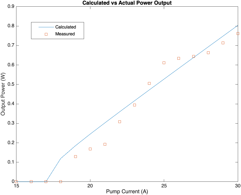
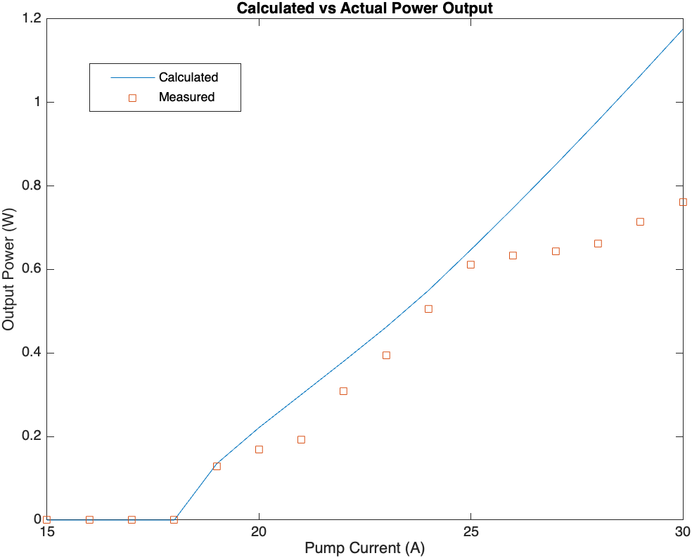
Thermal lensing causes the beam waist to become more focused in the KTP which increases its efficiency. But measurements don’t show that. One interesting data point here is that my measurements are taken immediately after the laser starts. I’ve noticed that the laser characteristics change rapidly within the first few seconds of operation. This is especially apparent when watching the pulses on an oscilloscope. My suspicion here is I am not actually measuring the effects of lensing. I’ve spot checked these values once they reach steady state and they still don’t match, however. Leaving the bench laser running for a while is not a good idea because I don’t have adequate cooling in the setup.
I am using the waist compression caused by thermal lensing in my design. I don’t have to “nail” this, but I have to get in the ballpark.
Next Steps
The parts to build the next bench setup should arrive Monday. The design holds some promise: the bench laser has no thermal control and loses half the second harmonic output due to the design. Factoring this in, it has already surpassed the power output of the 2020 laser with half the pump power.
Getting accurate second harmonic measurements is hard without good temperature control of the KTP crystal. Its rotation angle needs to be fixed for a certain temperature, and if the temperature changes the crystal rotation needs to match. Therefore you need to hold the crystal temperature constant to with about 0.1ºC. I don’t have the equipment needed for that on the bench.
Even without accurate measurements here I’m excited to see the results.